hypothesis test stata

Data Manipulation and Analysis in Stata

16 hypothesis tests, 16.1 for two categorical variables.

A common procedure is to test for an association between two categorical variables. We can illustrate this procedure using a tabulation with a \(\chi{}^2\) statistic. (Of course, the variable sex is not necessarily binary valued.)

16.2 Exercise

Create the table with \(\chi{}^2\) statistic and expected values as above. Should you reject the H0 that sex and class are not associated?

16.3 For one continuous and one categorical variable of two levels

If we have one continuous numeric variable and one two level categorical variable (such as employed vs unemployed) that would divide our data into two groups, we can ask ourselves whether the mean of the continuous variable differs for the groups (with H0 being that they do not).

If our two groups are independent, then we must first ask if the variance in the data is more or less equal between groups. The null hypothesis is that the variances are equal. This is tested by the comparison of variances using Stata’s robvar command. We can test the maths scores by sex in our data

Knowing whether or not we are dealing with groups displaying (more or less) equal variance in the variable of interest, we can go on to conduct an independent samples t-test . The code is

(Assuming that we have interpreted the results of robvar to mean the variance in maths for the two groups is equal).

16.4 Exercise

Run the robvar procedure above but for the history and sex variables. What are the three W statistics produced? Which of them tests that the variances are equal for a comparison of means? Is there strong enough evidence in this case to reject the null hypothesis?

Use the ttest command to test the null hypothesis that

\[\mu{}\ english _{\ female \ students} = \mu \ english _{\ male\ students}\]

What conclusion do you draw?

16.5 The paired samples ttest

We can also compare the same group of subjects on two measures to see if the means differ. In this case there is no need to check the variances before conducting the test. For example we could test whether or not mean scores in English and History differ (with the null hypothesis that they do not)

Using this procedure, how do English scores compare to History scores and how do English scores compare to Mathematics scores?

16.6 Once continuous and one categorical variable of more than two levels

We can compare the level avxm by teacher , this is to say test the null hypothesis

\[\mu{}\ avxm \ _{teacher \ one} = \mu{}\ avxm \ _{teacher \ two} = \mu{}\ avxm \ _{teacher \ three} \]

16.6.1 One way ANOVA and post-hoc testing

The Stata command to test the null hypothesis above is

This command produces summary statistics the ANOVA statistic F , its associated probability, and other quantities calculated as part of the ANOVA. In the version given above, we have included a tabulation of pairwise comparisons using the bonferroni correction. We can separately examine the pairwise comparisons if we wish with

This method does not display the ANOVA table itself and the mcompare() option gives us access to a slightly different range of correction options.

16.7 Two continuous variables

16.8 correlation.

Analysis of two continuous variables begins with calculating the Pearson Correlation Coefficient: R . This statistic ranges from

• -1 indicating an inverse or negative correlation
• 0 indicating no correlation
• +1 indicating a positive correlation

We should take note that a correlation has not only magnitude and direction, but that there is an associated hypothesis test: the the true correlation is 0. This test gives a p value associated with R .

The code to compute R in Stata is

This computes R for var1 and var2 . If you do not specify a variable list, Stata computes correlations between all non-string variables in your data set.

16.9 Exercise

Compute Pearson correlations with significance values for the pairs

• english-maths
• english-history

Explain to your learning partner what the results mean to you.

16.9.1 Simple visualisation of correlation

The simplest way to visualise a correlation is with a scatter plot. You may wish to consider, based on your plans for further analysis which variable you wish to assign to which axis. To create a scatter plot you can start with

To add the trend line:

And add a confidence interval:

Now you can add labels, titles and so on

Stata has a very large range of graphing commands and options. While they are reasonably complicated, a good way to explore them is through this gallery .

16.10 Exercise

Using any resources you can find, try to find more Stata graph schemes and try at least three on the code above.

An updated overview of multiple hypothesis testing commands in Stata

David mckenzie.

Just over a year ago, I wrote a blog post comparing different user-written Stata packages for conducting multiple hypothesis test corrections in Stata. Several of the authors of those packages have generously upgraded the commands to introduce more flexibility and cover more use cases, and so I thought I would provide an updated post that discusses the current versions. I’m also providing a sample dataset and do file that shows how I implemented the different commands. I again acknowledge my gratitude to the authors of these commands who have provided these public goods.

What is the problem we are trying to deal with here?

Suppose we have run an experiment with four treatments ( treat1, treat2, treat3, treat4 ), and are interested in examining impacts on a range of outcomes ( y1, y2, y3, y4, y5 ). In my empirical example here, the outcomes are firm survival (y1), and four different types of business practice indices (y2, y3, y4, and y5) and the treatments are different ways of helping firms learn new practices.

We run the following treatment regressions for outcome j:

Y(j) = a + b1*treat1+b2*treat2+b3*treat3+b4*treat4 + c1*y(j,0) + d’X + e(j)

Where here we have an Ancova specification, so control for the baseline value of the outcome variable in each regression y(j,0) – except for y1 (firm survival) since all firms were alive at time 0 and so there is no variation in the baseline value for this outcome; and control for randomization strata (the X’s here).

With 5 outcomes and 4 treatments, we have 20 hypothesis tests and thus 20 p-values, as shown in the table below:

Suppose that none of the treatments have any effect on any outcome (all null hypotheses are true), and that the outcomes are independent. Then if we just test the hypotheses one by one, then the probability that of one or more false rejections when using a critical value of 0.05 is 1-0.95^20 = 64% (and using a critical value of 0.10 is 88%. As a result, in order to reduce the likelihood of these false rejections, we want some way of adjusting for the fact that we are testing multiple hypotheses. That is what these different methods do.

Approaches for Controlling the False Discovery Rate (FDR): Anderson’s sharpened q-values

One of the most popular ways to deal with this issue is to use Michael Anderson’s code to compute sharpened False Discovery Rate (FDR) q-values. The FDR is the expected proportion of rejections that are type I errors (false rejections). Anderson discusses this procedure here .

This code is very easy to use. You need to just save the p-values and then read them as data into Stata, and run his code to get the sharpened q-values. For my little example, they are shown in the table below.

A few points to note:

·        A key reason for the popularity of this approach (in addition to its simplicity) is seen in the comparison of the original p-values to sharpened q-values. If we were to apply a Bonferroni adjustment, we would multiply the p-values by the number of outcomes (20) and then cap at 1.000. Then, for example, the p-value of 0.031 for outcome Y3 and treatment 1 would be adjusted to 0.62. Instead the sharpened q-value is 0.091. That is, this approach has a lot greater power than many other methods.

·        Because this takes the p-values as inputs, you have a lot of flexibility into what goes into each treatment regression: for example, you can have some regressions with clustered errors and some without, some with controls and some without, etc.

·        As Anderson notes in his code, sharpened q-values can actually be LESS than unadjusted p-values in some cases when many hypotheses are rejected, because if there are many true rejections, you can tolerate several false rejections too and still maintain the false discovery rate low.    We see an example of this for outcome Y1 and treatment 1 here.

·        A drawback of this method is that it does not account for any correlations among the p-values. For example, in my application, if a treatment improves business practices Y2, then we might think it is likely to have improved business practices Y3, Y4, and Y5. Anderson notes that in simulations the method seems to also work well with positively dependent p-values, but if the p-values have negative correlations, a more conservative approach is needed.

Approaches for Controlling the Familywise Error Rate (FWER)

An alternative to controlling the FDR is to control the familywise error rate (FWER), which is the probability of making any type I error. Many readers will be familiar with the Bonferroni correction noted above, which controls the FWER by adjusting the p-values by the number of tests. So if your p-value is 0.043, and you have done 20 tests, your adjusted p-value will be 20*0.043 = 0.86. As you can see, when the number of tests gets large, this correction can massively increase your p-values. Moreover, since it does not take account of any dependence among the outcomes, it can be way too conservative. All the methods I discuss here instead use a bootstrapping or re-sampling approach to incorporate information about the joint dependence structure of the different tests, thereby allowing p-values to be correlated and the adjusted p-values to be less conservative.

The table below adds FWER-adjusted p-values from four of these commands mhtexp, mhtreg, wyoung, and rwolf2 , all based on 3,000 bootstrap replications. I discuss each of these commands in turn, but you will see that:

·        All four methods give pretty similar adjusted p-values to one another here, with the small differences partly reflecting whether the method allows for different control variables to be used in each equation (discussed below).

·        While not as large as Bonferroni p-values would be, you can see the adjusted p-values are much larger than the original p-values and also typically quite a bit larger than the sharpened q-values. This reflects the issue of using FWER with many comparisons – in order to avoid making any type I error, the adjustments become increasingly severe as you add more and more outcomes or treatments. That is, power becomes low. In contrast, the FDR approach is willing to accept some type I error in exchange for more power. Which is more suitable depends on how costly false rejections are versus power to examine particular effects.

Let me then discuss the specifics of each of these four commands:

mhtexp (and mhtexp2)

This code implements a procedure set out by John List, Azeem Shaikh and Yang Xu (2016) , and can be obtained by typing ssc install mhtexp

List, Shaikh and Atom Vayalinka (2021) have an updated paper and code for mhtexp2 that builds in adjustment for baseline covariates using the Lin approach. It builds on work by Romano and Wolf, and uses a bootstrapping approach to incorporate information about the joint dependence structure of the different tests – that is, it allows for the p-values to be correlated.

·        This command allows for multiple outcomes and multiple treatments, but mhtexp does not allow for the inclusion of control variables (so no controlling for baseline values of the outcome of interest, or for randomization strata fixed effects), and does not allow for clustering of standard errors. mhtexp2 does allow for the inclusion of control variables, but currently requires them to be the same for every equation, and still does not allow for clustering of standard errors.

·        It assumes you are running simple treatment regressions, so does not allow for multiple testing adjustments coming from using e.g. ivreg, reghdfe, rdrobust, etc.

·        The command is then straightforward. Here I have created a variable treatment which takes value 0 for the control group, 1 for treat 1, 2 for treat 2, 3 for treat 3, and 4 for treat 4. Then the command is:

mhtexp Y1 Y2 Y3 Y4 Y5, treatment(treatment) bootstrap(3000)

So note that my mhtexp p-values above are from treatment regressions that don’t incorporate randomization strata fixed effects or the baseline values of the control variables.

This code was written by Andreas Steinmayr to extend the mhtexp command to allow for the inclusion of different controls in different regressions, and for clustered randomization.

To get this: type

ssc install mhtreg

A couple of limitations to be aware of:

·        The syntax is a bit awkward with multiple treatments – it only does corrections for the first regressor in each equation, so if you want to test for multiple treatments, you have to repeat the regression and change the order in which treatments are listed. E.g. to test the 20 different outcomes in my example, the code is:

·        It requires each treatment regression to actually be a regression – that is, to have used the reg command, and not commands like areg or reghdfe; or for you to be doing ivreg or probits, or something else – so you will need to add any fixed effects as regressors, and better be doing ITT and not TOT or other non-regression estimation.

This is one of the two commands that have improved the most since my first post, and it now does pretty much everything you would like it to do. This command, programmed by Julian Reif, calculates Westfall-Young stepdown adjusted p-values, which also control the FWER and allow for dependence amongst p-values. Documentation and latest updates are in the Github repository . It implements the Westfall-Young method, which uses bootstrap resampling to allow for dependence across outcomes. This method is a precursor to the Romano-Wolf procedure that the other three commands I note here are based on. Romano and Wolf note that the Westfall-Young procedure requires an additional assumption of subset pivotality, which can be violated in certain settings, and so the Romano-Wolf procedure is more general.   For multiple test correction with OLS and experimental analysis, this assumption should hold fine, and as we see in my example, both methods give similar results here.

To get this command, type

net install wyoung, from(" https://raw.githubusercontent.com/reifjulian/wyoung/master ") replace

·        A nice feature of this command is that it allows you to have different control variables in different equations. So you can control for the baseline variable of each outcome, for example. It also allows for clustered randomization and can do bootstrap re-sampling that accounts for both randomization strata and clustered assignment.

·        The command allows for different Stata commands in different equations – so you could have one equation be estimated using IV, another using reghdfe, another with a regression discontinuity, etc

·        The updates made now allow for multiple treatments and for a much cleaner syntax for including different control variables in different regressions. One point to note is that if there is an equation where you do not want to include a control, but you do want to include controls in others, the current command seems to require a hack where you just create a constant as the control variable for the equations where you do not want controls.

gen constant=1

wyoung Y1 Y2 Y3 Y4 Y5, cmd(areg OUTCOMEVAR treat1 treat2 treat3 treat4 CONTROLVARS, r a(strata)) familyp(treat1 treat2 treat3 treat4) controls("constant" "b_Y2" "b_Y3" "b_Y4" "b_Y5") bootstraps(1000) seed(123);

#delimit cr

This command calculates Romano-Wolf stepdown adjusted p-values, which control the FWER and allows for dependence among p-values by bootstrap resampling. The original rwolf command was developed by Romano and Wolf along with Damian Clarke. It is the command that I think has improved the most with the recent update by Damian Clarke to rwolf2 , described here . The updates expand the capabilities of the command to deal with what I saw as the main limitations of the original command, and it now allows for multiple treatments, different commands, different controls in different regressions, and also allows for clustered standard errors. Here is an example of the syntax:

Since this now does everything that the Westfall-Young command does, while been able to handle cases where subset pivotality does not hold, then this currently seems the theoretically best option for FWER correction at the moment.

Testing the null of complete irrelevance: randcmd

This is a Stata command written by Alwyn Young that calculates randomization inference p-values, based on his recent QJE paper . It is doing something different to the above approaches. Rather than adjusting each individual p-value for multiple testing, it conducts a joint test of the sharp hypothesis that no treatment has any effect, and then uses the Westfall-Young approach to test this across equations. So in my example, it tests that there is no effect of any treatment on outcome Y1 (p=0.403), Y2 (p=0.0.045) etc., and then also tests the null of complete irrelevance – that no treatment had no effect on any outcome (p=0.022 here). The command is very flexible in allowing for each equation to have different controls, different samples, having clustered standard errors, etc. But it is testing a different hypothesis than the other approaches above.

Putting it altogether

The table below summarizes the different multiple hypothesis testing commands. With a small number of hypothesis tests, controlling for the FWER is useful, and then both rwolf2 and wyoung do everything you need. With lots of outcomes and treatments, controlling for the FDR is likely to be preferred in many economics applications, and so the Anderson q-value approach is my stand-by. The Young omnibus test of overall significance is a useful compliment, but answers a different question.

Get updates from Development Impact

Thank you for choosing to be part of the Development Impact community!

Your subscription is now active. The latest blog posts and blog-related announcements will be delivered directly to your email inbox. You may unsubscribe at any time.

Lead Economist, Development Research Group, World Bank

Join the Conversation

• Share on mail
• comments added

• [email protected]
• Connecting and sharing with us

• Entrepreneurship
• Growth of firm
• Sales Management
• Retail Management
• Import – Export
• International Business
• Project Management
• Production Management
• Quality Management
• Logistics Management
• Supply Chain Management
• Human Resource Management
• Organizational Culture
• Information System Management
• Corporate Finance
• Stock Market
• Office Management
• Theory of the Firm
• Management Science
• Microeconomics
• Research Process
• Experimental Research
• Research Philosophy
• Management Research
• Writing a thesis
• Writing a paper
• Literature Review
• Action Research
• Qualitative Content Analysis
• Observation
• Phenomenology
• Statistics and Econometrics
• Questionnaire Survey
• Quantitative Content Analysis
• Meta Analysis

Hypothesis Tests with Linear Regression by using Stata

Two types ofhypothesis tests appear in regress output tables. As with other common hypothesis tests, they begin from the assumption that observations in the sample at hand were drawn randomly and independently from an infinitely large population.

• Overall F test: The F statistic at the upper right in the regression table evaluates the null hypothesis that in the population, coefficients on all the model’s x variables equal zero.
• Individual t tests: The third and fourth columns of the regression table contain t tests for each individual regression coefficient. These evaluate the null hypotheses that in the population, the coefficient on each particular x variable equals zero.

The t test probabilities are two-sided. For one-sided tests, divide these p-values in half.

In addition to these standard F and t tests, Stata can perform F tests of user-specified hypotheses. The test command refers back to the most recently fitted model such as anova or regress. Returning to our four-predictor regression example, suppose we with to test the null hypothesis that both adfert and chldmort (considered jointly) have zero effect.

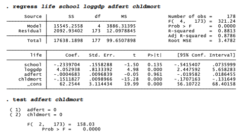
While the individual null hypotheses point in opposite directions (effect of chldmort significant, adfert not), the joint hypothesis that coefficients on chldmort and adfert both equal zero can reasonably be rejected (p < .00005). Such tests on subsets of coefficients are useful when we have several conceptually related predictors or when individual coefficient estimates appear unreliable due to multicollinearity.

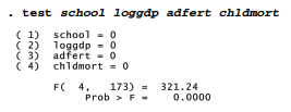
test could duplicate the overall F test:

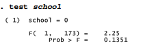
test also could duplicate the individual-coefficient tests. Regarding the coefficient on school, for example, the F statistic obtained by test equals the square of the t statistic in the regression table, 2.25 = (-1.50) 2 , and yields exactly the same p-value:

Applications of test more useful in advanced work (although not meaningful for the life- expectancy example at hand) include the following.

• Test whether a coefficient equals a specified constant. For example, to test the null hypothesis that the coefficient on school equals 1 (H 0 😛 1 = 1), instead of testing the usual null hypothesis that it equals 0 (H 0 😛 1 = 0), type

. test school = 1

• Test whether two coefficients are equal. For example, the following command evaluates the null hypothesis H 0 😛 2 = P 3

. test loggdp = adfert

• Finally, test understands some algebraic expressions. We could request something like the following, which would test H 0 😛 2 = (P 3 + P 4 ) / 100

. test school = (loggdp + adfert)/100

Consult help test for more information and examples.

Source: Hamilton Lawrence C. (2012), Statistics with STATA: Version 12 , Cengage Learning; 8th edition.

23 Sep 2022

24 Sep 2022

1 thoughts on “ Hypothesis Tests with Linear Regression by using Stata ”

I haven?¦t checked in here for some time because I thought it was getting boring, but the last few posts are good quality so I guess I will add you back to my daily bloglist. You deserve it my friend 🙂

Leave a Reply Cancel reply

Your email address will not be published. Required fields are marked *

Save my name, email, and website in this browser for the next time I comment.

Username or email address  *

Password  *

Log in Remember me

Lost your password?

A GUIDE TO APPLIED STATISTICS WITH STATA

Statistical hypothesis testing.

Written by:

Ylva B Almquist

Conducting a statistical hypothesis test is easy to do in statistical software such as Stata. These tests give us a probability value (p-value) that can help us decide whether or not the null hypothesis should be rejected. See P-values for a further discussion.

• Skip to primary navigation
• Skip to main content
• Skip to primary sidebar

Statistical Methods and Data Analytics

How can I perform the likelihood ratio and Wald test in Stata? | Stata FAQ

Purpose:  This page shows you how to conduct a likelihood ratio test and Wald test in Stata. For a more conceptual understanding, including an explanation of the score test, refer to  the FAQ page How are the likelihood ratio, Wald, and Lagrange multiplier (score) tests different and/or similar?

The likelihood ratio (LR) test and Wald test test are commonly used to evaluate the difference between nested models. One model is considered nested in another if the first model can be generated by imposing restrictions on the parameters of the second. Most often, the restriction is that the parameter is equal to zero. In a regression model restricting a parameters to zero is accomplished by removing the predictor variables from the model. For example, in the models below, the model with the predictor variables female , and read , is nested within the model with the predictor variables female , read , math , and science . The LR and Wald ask the same basic question, which is, does constraining these parameters to zero (i.e., leaving out these predictor variables) significantly reduce the fit of the model? To perform a likelihood ratio test, one must estimate both of the models one wishes to compare. The advantage of the Wald test is that it approximates the LR test but require that only one model be estimated. When computing power was much more limited, and many models took a long time to run, this was a fairly major advantage. Today, for most of the models researchers are likely to want to compare, this is not an issue, and we generally recommend running the likelihood ratio test in most situations. This is not to say that one should never use the Wald test. For example, the Wald test is commonly used to perform multiple degree of freedom tests on sets of dummy variables used to model categorical variables in regression (for more information see our webbook on Regression with Stata, specifically Chapter 3 – Regression with Categorical Predictors ).

As we mentioned above, the LR test requires that two models be run, one of which has a set of parameters (variables), and a second model with all of the parameters from the first, plus one or more other variables. The Wald test examines a model with more parameters and assess whether restricting those parameters (generally to zero, by removing the associated variables from the model) seriously harms the fit of the model. In general, both tests should come to the same conclusion (because the Wald test, at least in theory, approximate the LR test). As an example, we will test for a statistically significant difference between two models, using both tests.

The dataset for this example includes demographic data, as well as standardized test scores for 200 high school students. We will compare two models. The dependent variable for both models is hiwrite (to be nested two models must share the same dependent variable), which is a dichotomous variable indicating that the student had a writing score that was above the mean. There are four possible predictor variables, female , a dummy variable which indicates that the student is female, and the continuous variables read , math , and science , which are the student’s standardized test scores in reading, math, and science, respectively. We will test a model containing just the predictor variables female and read , against a model that contains the predictor variables female and read , as well as, the additional predictor variables, math and science .

Example of a likelihood ratio test.

As discussed above, the LR  test involves estimating two models and comparing them. Fixing one or more parameters to zero, by removing the variables associated with that parameter from the model, will almost always make the model fit less well, so a change in the log likelihood does not necessarily mean the model with more variables fits significantly better. The LR test compares the log likelihoods of the two models and tests whether this difference is statistically significant. If the difference is statistically significant, then the less restrictive model (the one with more variables) is said to fit the data significantly better than the more restrictive model. The LR test statistic is calculated in the following way:

$$LR = -2 ln\left(\frac{L(m_1)}{L(m_2)}\right) = 2(loglik(m_2)-loglik(m_1))$$

Where $L(m_*)$ denotes the likelihood of the respective model (either Model 1 or Model 2), and $loglik(m_*)$ the natural log of the model’s final likelihood (i.e., the log likelihood). Where $m_1$ is the more restrictive model, and $m_2$ is the less restrictive model.

This statistic is distributed chi-squared with degrees of freedom equal to the difference in the number of degrees of freedom between the two models (i.e., the number of variables added to the model).

In order to perform the likelihood ratio test we will need to run both models and make note of their final log likelihoods. We will run the models using Stata and use commands to store the log likelihoods. We could also just copy the likelihoods down (i.e., by writing them down, or cutting and pasting), but using commands is a little easier and is less likely to result in errors. The first line of syntax below reads in the dataset from our website. The second line of syntax runs a logistic regression model, predicting hiwrite based on students’ gender ( female ), and reading scores ( read ). The third line of code stores the value of the log likelihood for the model, which is temporarily stored as the returned estimate e(ll) (for more information type help return in the Stata command window), in the scalar named m1 .

use https://stats.idre.ucla.edu/stat/stata/faq/nested_tests, clear logit hiwrite female read scalar m1 = e(ll)

Below is the output. In order to perform the likelihood ratio test we will need to keep track of the log likelihood (-102.44), the syntax for this example (above) does this by storing the value in a scalar. Since it is not our primary concern here, we will skip the interpretation of the rest logistic regression model. Note that storing the returned estimate does not produce any output.

Iteration 0: log likelihood = -137.41698 Iteration 1: log likelihood = -104.79885 Iteration 2: log likelihood = -102.52269 Iteration 3: log likelihood = -102.44531 Iteration 4: log likelihood = -102.44518 Logistic regression Number of obs = 200 LR chi2(2) = 69.94 Prob > chi2 = 0.0000 Log likelihood = -102.44518 Pseudo R2 = 0.2545 ------------------------------------------------------------------------------ hiwrite | Coef. Std. Err. z P>|z| [95% Conf. Interval] -------------+---------------------------------------------------------------- female | 1.403022 .3671964 3.82 0.000 .6833301 2.122713 read | .1411402 .0224042 6.30 0.000 .0972287 .1850517 _cons | -7.798179 1.235685 -6.31 0.000 -10.22008 -5.376281 ------------------------------------------------------------------------------

The first line of syntax below runs the second model, that is, the model with all four predictor variables. The second line of code stores the value of the log likelihood for the model (-84.4), which is temporarily stored as the returned estimate ( e(ll) ), in the scalar named m2 . Again, we won’t say much about the output except to note that the coefficients for both math and science are both statistically significant. So we know that, individually, they are statistically significant predictors of hiwrite .

logit hiwrite female read math science scalar m2 = e(ll) Iteration 0: log likelihood = -137.41698 Iteration 1: log likelihood = -90.166892 Iteration 2: log likelihood = -84.909776 Iteration 3: log likelihood = -84.42653 Iteration 4: log likelihood = -84.419844 Iteration 5: log likelihood = -84.419842 Logistic regression Number of obs = 200 LR chi2(4) = 105.99 Prob > chi2 = 0.0000 Log likelihood = -84.419842 Pseudo R2 = 0.3857 ------------------------------------------------------------------------------ hiwrite | Coef. Std. Err. z P>|z| [95% Conf. Interval] -------------+---------------------------------------------------------------- female | 1.805528 .4358101 4.14 0.000 .9513555 2.6597 read | .0529536 .0275925 1.92 0.055 -.0011268 .107034 math | .1319787 .0318836 4.14 0.000 .069488 .1944694 science | .0577623 .027586 2.09 0.036 .0036947 .1118299 _cons | -13.26097 1.893801 -7.00 0.000 -16.97275 -9.549188 ------------------------------------------------------------------------------

Now that we have the log likelihoods from both models, we can perform a likelihood ratio test. The first line of syntax below calculates the likelihood ratio test statistic. The second line of syntax below finds the p-value associated with our test statistic with two degrees of freedom. Looking below we see that the test statistic is 36.05, and that the associated p-value is very low (less than 0.0001). The results show that adding math and science as predictor variables together (not just individually) results in a statistically significant improvement in model fit. Note that if we performed a likelihood ratio test for adding a single variable to the model, the results would be the same as the significance test for the coefficient for that variable presented in the above table.

di "chi2(2) = " 2*(m2-m1) di "Prob > chi2 = "chi2tail(2, 2*(m2-m1)) chi2(2) = 36.050677 Prob > chi2 = 1.485e-08

Using Stata’s postestimation commands to calculate a likelihood ratio test

As you  have seen, it is easy enough to calculate a likelihood ratio test “by hand.” However, you can also use Stata to store the estimates and run the test for you. This method is easier still, and probably less error prone. The first line of syntax runs a logistic regression model, predicting hiwrite based on students’ gender ( female ), and reading scores ( read ). The second line of syntax asks Stata to store the estimates from the model we just ran, and instructs Stata that we want to call the estimates m1 . It is necessary to give the estimates a name, since Stata allows users to store the estimates from more than one analysis, and we will be storing more than one set of estimates.

use https://stats.idre.ucla.edu/stat/stata/faq/nested_tests, clear logit hiwrite female read estimates store m1

Below is the output. Since it is not our primary concern here, we will skip the interpretation of the logistic regression model. Note that storing the estimates does not produce any output.

Iteration 0:   log likelihood = -137.41698-137.41698-137.41698 Iteration 1:   log likelihood = -104.79885 Iteration 2:   log likelihood = -102.52269 Iteration 3:   log likelihood = -102.44531 Iteration 4:   log likelihood = -102.44518 Logistic regression                               Number of obs   =        200                                                   LR chi2(2)      =      69.94                                                   Prob > chi2     =     0.0000 Log likelihood = -102.44518                       Pseudo R2       =     0.2545 ------------------------------------------------------------------------------      hiwrite |      Coef.   Std. Err.      z    P>|z|     [95% Conf. Interval] -------------+----------------------------------------------------------------       female |   1.403022   .3671964     3.82   0.000     .6833301    2.122713         read |   .1411402   .0224042     6.30   0.000     .0972287    .1850517        _cons |  -7.798179   1.235685    -6.31   0.000    -10.22008   -5.376281 ------------------------------------------------------------------------------

The first line of syntax below this paragraph runs the second model, that is the model with all four predictor variables. The second line of syntax saves the estimates from this model, and names them m2 . Below the syntax is the output generated. Again, we won’t say much about the output except to note that the coefficients for both math and science are both statistically significant. So we know that, individually, they are statistically significant predictors of hiwrite . The tests below will allow us to test whether adding both of these variables to the model significantly improves the fit of the model, compared to a model that contains just female and read .

logit hiwrite female read math science estimates store m2 Iteration 0:   log likelihood = -137.41698 Iteration 1:   log likelihood = -90.166892 Iteration 2:   log likelihood = -84.909776 Iteration 3:   log likelihood =  -84.42653 Iteration 4:   log likelihood = -84.419844 Iteration 5:   log likelihood = -84.419842 Logistic regression                               Number of obs   =        200                                                   LR chi2(4)      =     105.99                                                   Prob > chi2     =     0.0000 Log likelihood = -84.419842                       Pseudo R2       =     0.3857 ------------------------------------------------------------------------------      hiwrite |      Coef.   Std. Err.      z    P>|z|     [95% Conf. Interval] -------------+----------------------------------------------------------------       female |   1.805528   .4358101     4.14   0.000     .9513555      2.6597         read |   .0529536   .0275925     1.92   0.055    -.0011268     .107034         math |   .1319787   .0318836     4.14   0.000      .069488    .1944694      science |   .0577623    .027586     2.09   0.036     .0036947    .1118299        _cons |  -13.26097   1.893801    -7.00   0.000    -16.97275   -9.549188 ------------------------------------------------------------------------------

The first line of syntax below tells Stata that we want to run an lr test, and that we want to compare the estimates we have saved as m1 to those we have saved as m2 . The output reminds us that this test assumes that A is nested in B, which it is. It also gives us the chi-squared value for the test (36.05) as well as the p-value for a chi-squared of 36.05 with two degrees of freedom. Note that the degrees of freedom for the lr test, along with the other two tests, is equal to the number of parameters that are constrained (i.e., removed from the model), in our case, 2. Note that the results are the same as when we calculated the lr test by hand above. Adding math and science as predictor variables together (not just individually) results in a statistically significant improvement in model fit. As noted when we calculated the likelihood ratio test by hand, if we performed a likelihood ratio test for adding a single variable to the model, the results would be the same as the significance test for the coefficient for that variable presented in the table above.

lrtest m1 m2 Likelihood-ratio test                                  LR chi2(2)  =     36.05 (Assumption: A nested in B)                            Prob > chi2 =    0.0000

The entire syntax for a likelihood ratio test, all in one block, looks like this:

logit hiwrite female read estimates store m1 logit hiwrite female read math science estimates store m2 lrtest m1 m2

Example of a Wald test

As was mentioned above, the Wald test approximates the LR test, but with the advantage that it only requires estimating one model. The Wald test works by testing that the parameters of interest are simultaneously equal to zero. If they are, this strongly suggests that removing them from the model will not substantially reduce the fit of that model, since a predictor whose coefficient is very small relative to its standard error is generally not doing much to help predict the dependent variable.

The first step in performing a Wald test is to run the full model (i.e., the model containing all four predictor variables). The first line of syntax below does this (but uses the quietly prefix so that the output from the regression is not shown). The second line of syntax below instructs Stata to run a Wald test in order to test whether the coefficients for the variables math and science are simultaneously equal to zero. The output first gives the null hypothesis. Below that we see the chi-squared value generated by the Wald test, as well as the p-value associated with a chi-squared of 27.53 with two degrees of freedom. Based on the p-value, we are able to reject the null hypothesis, again indicating that the coefficients for math and science are not simultaneously equal to zero, meaning that including these variables create a statistically significant improvement in the fit of the model.

Your Name (required)

Your Email (must be a valid email for us to receive the report!)

Comment/Error Report (required)

How to cite this page

• © 2024 UC REGENTS